causal models cannot explain quantum predictions in extended Wigner’s friend scenarios
A couple of weeks ago one of my favourite projects (Yīng et al. 2024) got published in Quantum! There we (Yìlè Yīng, Marina Maciel Ansanelli, Elie Wolfe, David Schmid, Eric Cavalcanti, and I) show how Wigner’s friend thought experiments challenge nonclassical causal reasoning.
We show that our most powerful frameworks for causal reasoning are incapable of producing a good account of quantum mechanical predictions if one assumes that:
- observers have single definite experiences at all times
- quantum mechanics can be applied to any system
The result is simple enough to state, but to understand it, one has to cover quite some background, which you can also find in the paper. Here I will do a shorter, easier, and (needless to say!) less careful version of it here. I’ll inevitably leave some nuance out, but by reading this you will get the main gist.
I will first cover some necessary background: classical causal reasoning, and its failure to account for quantum mechanical predictions (in particular Bell inequality violations), the concept of finetuning, and the introduction of (post-)quantum causal modelling as a response. Then we will talk about the Extended Wigner’s friend scenario and the local friendliness no-go theorem. After covering all this material, stating our result will be as simple as saying:
all GPT causal explanations of Local Friendliness inequality violations (that assign an observed variable to the friends) are finetuned.
You can also watch my friend and co-author Yìlè Yīng’s presentation at Causalworlds 2024 about it (watch it here), and also have a look at my poster (pdf) for the Vienna Quantum Foundations conference.
Let’s get started.
Bell as a challenge to classical causal reasoning
There are several ways to understand the implications of Bell inequality violations, but one of my favourite is definitely due to Christopher Wood and Robert Spekkens (Wood and Spekkens 2015). In this seminal paper, they showed how Bell inequality violations mean that classical causal reasoning fails to account for the data collected in quantum experiments, and introduced a framework of quantum causal reasoning that instead can account for these predictions.
In classical causal reasoning we postulate a causal structure in the form of a directed acyciclic graph (DAG) that relates causes and effects. To each graph we associate a family of probability distributions that are compatible with it. This is done by specifying its functional form via the so-called Markov condition. Intuitively, the Markov condition ensures that each variable’s statistics only directly depend on its immediate causes. In more precise terms, conditioning on the immediate causes of a variable should decorrelate that variable from all the others. It’s easier to see with an example, which we will do in a second.
Let me just say that this framework, devised and popularised for example by Judea Pearl (Pearl 2000), besides providing a clear and workable notion of cause and effect (an important philosophical question), has been used with success in many fields such as engineering, ai, medicine, economics. Sometimes knowing the difference between causation and correlation is a matter of literal life or death, and this is where classical causal reasoning comes to the rescue.
It’s good stuff. But it’s not enough when quantum mechanics gets involved.
the obvious explanation doesn’t work
If i describe to you a Bell experiment, you would draw this graph:
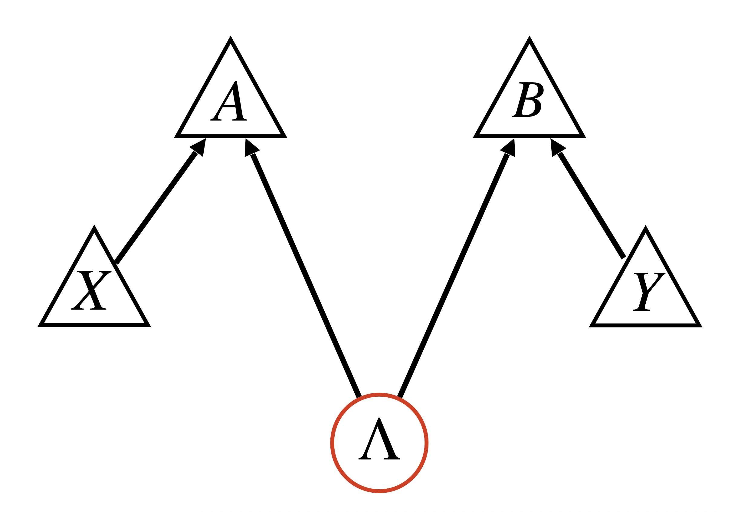
Let’s call it the Bell DAG. Here, and are the measurement outcomes, and are the measurement inputs, and is some latent variable associated to the source. Arrows point from cause to effect. The situation is simple here: the outcome can be causally affected by the experimental setting and the apparatus that distributes the photons, but not by the setting in the other lab or the outcome there. Why would it?
The Markov condition restricts the probability distributions for the observed variables to have the following functional form:
the probabilities on the RHS are unconstrained, but this constrains the possible distributions on the LHS.
In particular, this equation implies that cannot violate the Bell inequalities. All probability distributions compatible with this causal structure have to satisfy the Bell inequalities, no matter what the values of the $p$ on the right hand side.
Bell’s theorem could be formulated as follows: If you described a Bell experiment to a statistician, they would draw a Bell DAG, but if instead you gave them just the data, they would rule out this causal structure, as it is incompatible with the data.
But that is not all, indeed the best is yet to come.
all explanations are bad
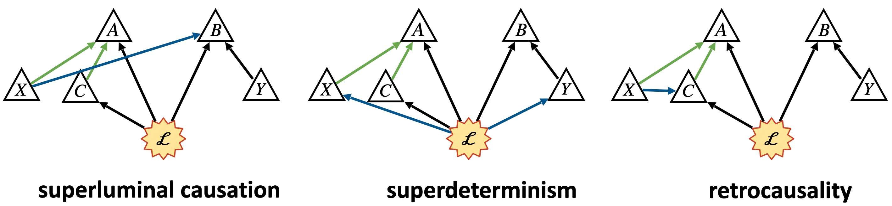
Of course there are some causal structures which allow for a classical causal explanation, just add some causal arrow here or there. Here are some examples:
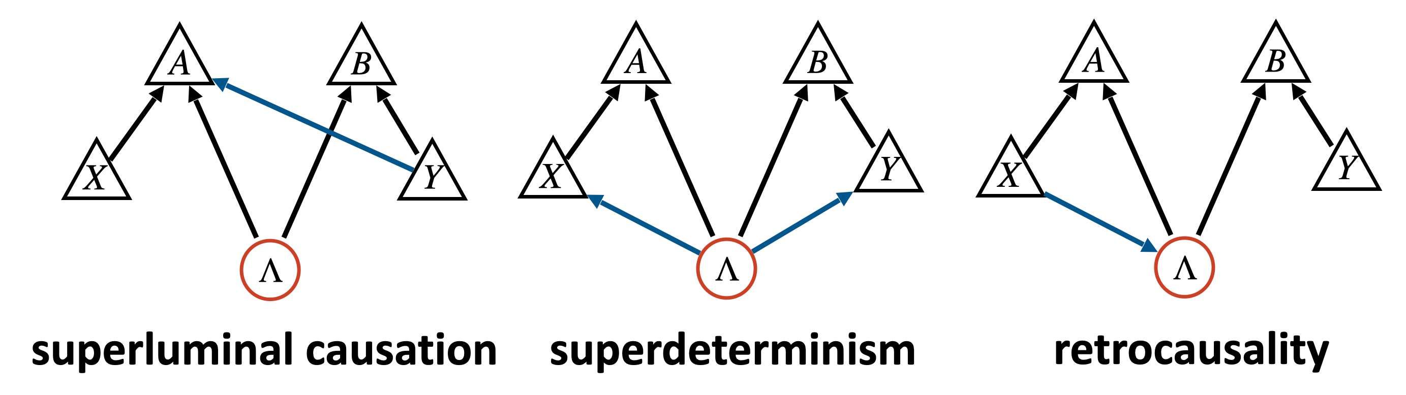
The probability distributions that are Markov-compatible with these DAGs can violate the Bell inequalities. Indeed, all these causal structures have been presented as solutions to the Bell inequality violations.
These causal explanations are in severe tension with relativity, thermodynamics, and/or our causal sensibilities. But they are bad in an independent, technical, sense: they are finetuned. (I’ll say in a moment what that means, but let me say this: finetuning is a concept native to the field of causal inference and has nothing to do with relativity.)
The actual big statement of Wood and Spekkens is the following:
all classical causal explanations of Bell inequality violations are finetuned
So, not only is the most obvious classical causal model for the Bell experiment unable to account for the data, all classical causal models that can reproduce the data are in fact bad explanations, in a precise technical sense. Ouch.
At the bottom of this blog, I explain what finetuning is, and why it is bad. I put it at the bottom because it’s a bit long. If you need the details, go ahead and read it; otherwise just take my word for it for the moment. The main idea is that the model’s parameters (the specific conditional probability distributions between variables and their direct causes) have to be selected very carefully to hide the extra arrows which are invisible in the data.
I should also mention that finetuning is not a coup the grâce for the model: your theory simply has to provide an explanation for these parameters. This is case of Bohmian mechanics, which uses a finetuned superluminal causal influence which is hidden by the so-called quantum equilibrium condition. But Bohmian mechanics also provides an explanation for this equilibrium, so it’s fine.1 Superdeterministic models don’t do this, as far as I’m aware.
the solution: quantum causal models
So we have no good classical causal account for Bell inequality violations. What to do?
Let’s introduce quantum causal modelling! Replace a classical common cause with a quantum common cause.
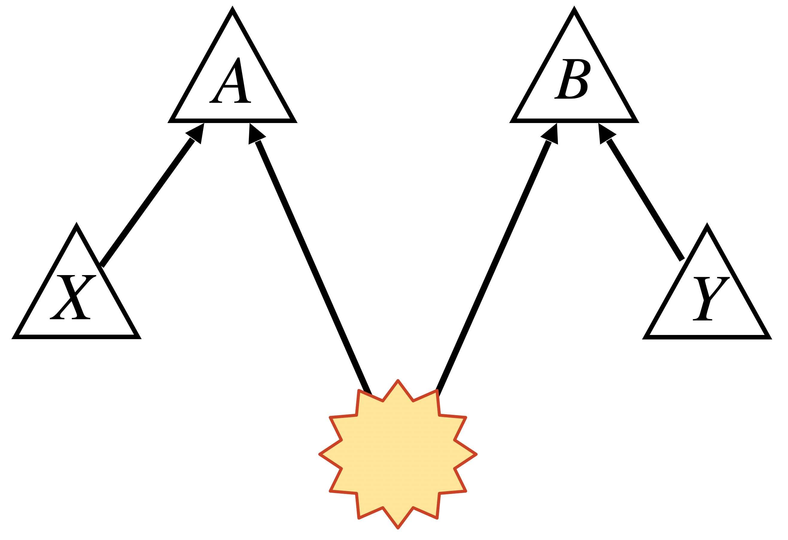
where is a density operator on a composite quantum system and, for each value of and , and are POVMs on and , respectively.
Of course such a distribution can violate the Bell inequalities. We get a non-finetuned causal account for our data—in harmony with relativity!
bye bye Reichenbach
Ok what’s the catch? We had to modify our very notion of common cause: we sacrificed Reichenbach’s principle of common cause (Reichenbach 1999). This is two ideas packaged together.
The first one is: if there is a correlation between two variables and then either one is the cause of the other, or there is a common cause explaining the correlations. This sounds so basic we hardly want to state it, but it is, indeed, a postulate. The other part is that to explain a correlation means that conditioning on removes the correlation between and . This is the idea of a decorrelating explanation. This is precisely what we lose when we move from classical causal models to quantum causal models. In the example above, knowing the state does not remove the correlations between and
If the principle of decorrelating explanation does not sound natural to you, it might be because it does not hold in quantum mechanics, and maybe you have absorbed the quantum way of looking at things. But I guarantee you, if you think about it for a bit in the context of classical logic, you’ll realise its quite natural.
If you want to know more about this—and also if you want to really understand Bell—read this classic: (Wiseman and Cavalcanti 2015).
post-quantum causal models are not enough
Quantum causal modelling/inference/discovery is a whole field now, it can be used to explain all sorts of experiments, certify the effectiveness of your quantum cryptography protocols, design post-quantum ready cryptography and so on. It’s one of the main research directions at Perimeter Institute; see, for example this talk by Rob Spekkens and Elie Wolfe.
It has also been generalised to Generalised Probabilistic Theories (GPTs) (Henson, Lal, and Pusey 2014), where the latent nodes can be as exotic as PR boxes or even more.
If you don’t know what GPTs are don’t worry. GPTs are theories like quantum mechanics and classical information theory, where you have systems, states, measurements, and probabilities. They are useful in quantum foundations to understand what is special about classical or quantum, to investigate possible new theories, to formulate no-go theorems etc. You can read just a little and find good references in (Di Biagio 2024).
So, with all this power, we should be able to explain everything, surely? This is where Wigner—and our paper—comes on stage.
extended Wigner’s friend scenario
The extended Wigner’s friend scenario (EWFS) is a marriage of Wigner’s friend thought experiment and Bell’s experiment. It is in fact a whole family of different thought experiments, where you have some observers (the “friends”) interacting with some simple quantum systems, and some superobservers (the “wigners”) who—by assumption—have complete quantum control over their friends and who might perform some quantum interference experiments on their friends. If the quantum systems are entangled one can get quite striking results. The papers that brought into focus the power of these extended Wigner’s friends scenario have just been awarded the Paul Ehrenfest prize by IQOQI Vienna. See (Schmid, Yīng, and Leifer 2023) for a review.
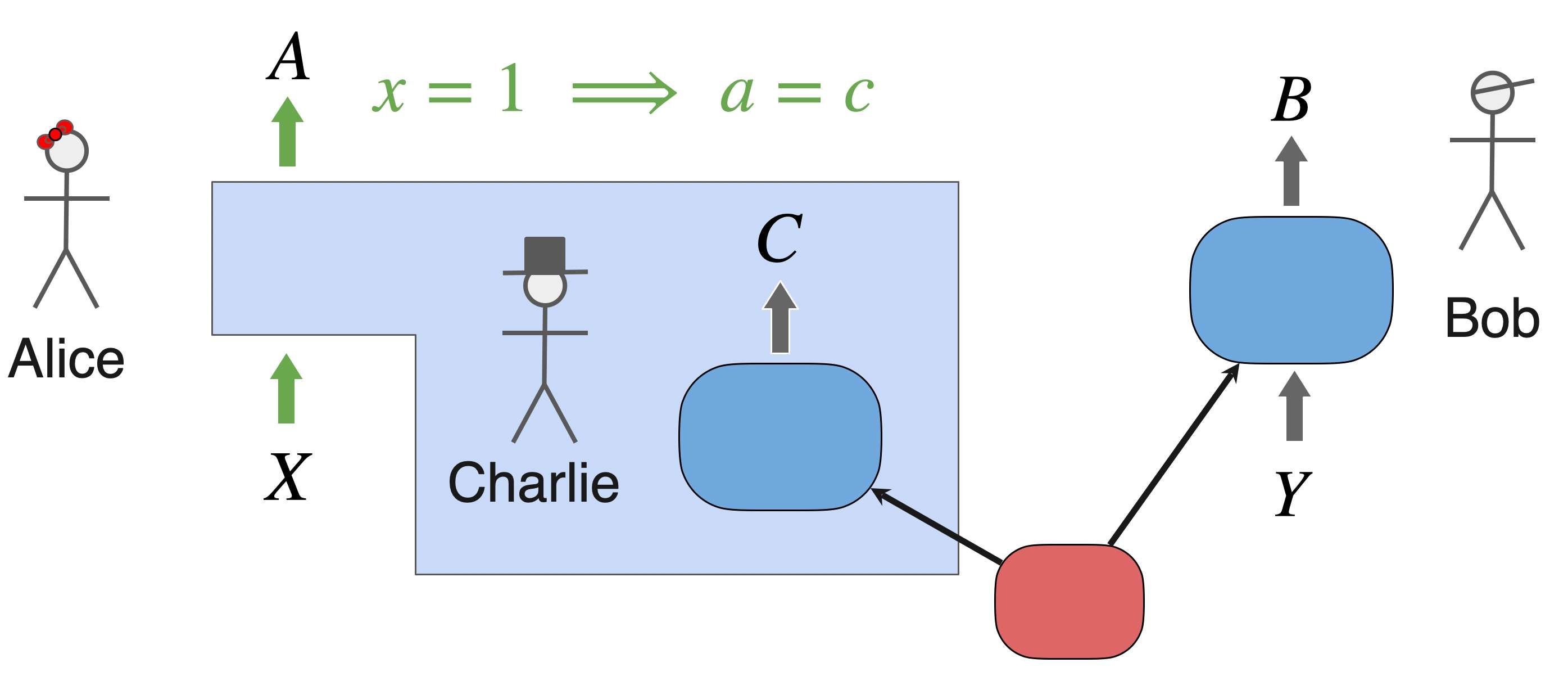
We will consider for simplicity the minimal EWFS. We have three agents, Alice, Bob, and Charlie. Alice has inputs and outputs , Bob has and Charlie always only has output . Charlie and Bob both perform a measurement on their half of an entangled system
Here comes the “Wigner” twist: Alice has full quantum control over Charlie, and she describes Charlie’s interaction with his system as a unitary evolution that entangles him (and his lab) with the quantum system. If , she just “opens the box” and copies Charlie’s result. Otherwise she coherently reverses the unitary that entangled him with his system (hopefully she got consent!) and does a measurement on the system directly, on a basis complementary to the one Charlie did.
Turns out there is a Bell-like no-go theorem for this setup (Bong et al. 2020). In fact, a stronger no-go theorem than Bell, as it relies on weaker assumptions. It’s called the Local Friendliness (LF) no-go theorem. Let’s review it quickly.
the local friendliness inequalities
Let’s make explicit an assumption already implicitly present in Bell: absoluteness of observed events. AOE means that observers have definite outcomes and that these outcomes can be communicated. If you additionally assume no-superdeterminism and locality, you obtain2 a set of constraints on the statistics of Alice and Bob’s measurements known as the Local Friendliness inequalities.
But we know that, if QM can be applied to Charlie, then we know that we can set up an experiment where Alice and Bob can violate the LF inequalities!
Hence the no-go theorem: the assumption that QM holds for arbitrarily large systems is in contradiction with AOE, no superdeterminism, and locality.
Of course to do a minimal extended Wigner’s friend experiment with an actual person is (probably) science fiction. But is it a practical, or fundamental limitation? Quantum mechanics does not tell us where unitary evolution is supposed to stop, and we’ve been doing interference experiments and confirming QM’s predictions with larger and larger systems (Fein et al. 2019). The LF inequalities have already been violated with several qubits acting as a “friend” (Zeng, Labib, and Russo 2024), and it’s totally conceivable we’ll be able to do it with an AGI in a quantum computer (Wiseman, Cavalcanti, and Rieffel 2023).
I think we should take this seriously. All interpretations that held onto no superdeterminism and locality in the face of Bell have to face this theorem. This includes most (neo-)Copenhagen interpretations (those that were comfortable with modifying Reichenbach’s principle). They basically either have to proclaim that QM fails at some point, or get serious about AOE.
our main result: bad post-quantum causal explanations
This is the causal structure you would draw given the description of the experiment:
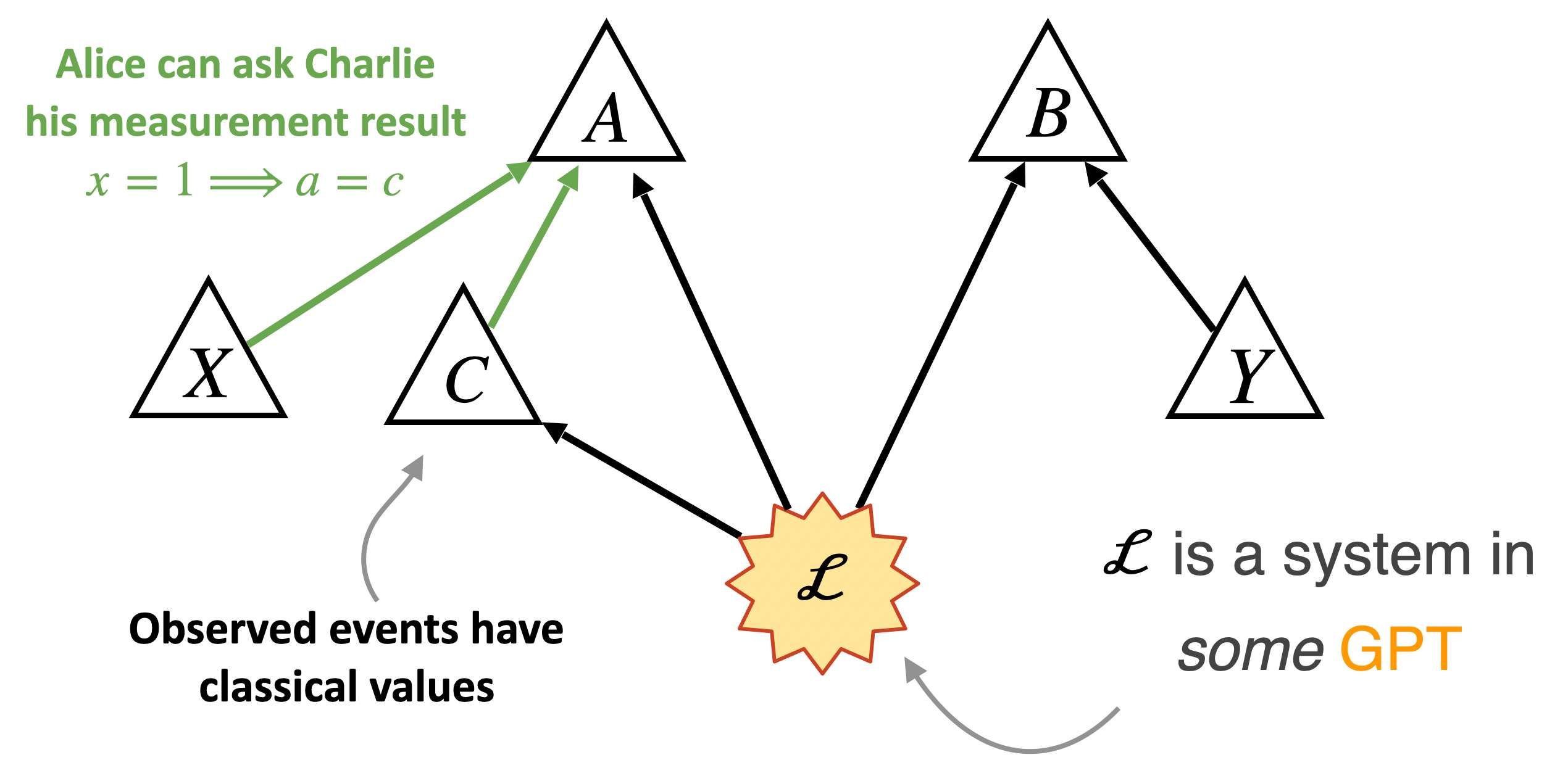
Let’s call if the LF DAG. Here, the node for is a classical variable, since it is an observed variable, and we are assuming that observations should have definite outcomes.
In GPT causal modelling, the Markov condition, which told you which probability distributions are classically compatible with a given DAG, is replaced by a generalised Markov condition, which tells you how to draw a GPT circuit compatible with the causal structure, and then the circuit itself tells you which probabilities are possible. The details are not too important; you can check appendix A of our paper if you want to know more.
The generalised Markov condition implies that probability distributions compatible with the LF DAG have to satisfy the local friendliness inequalities!
Not only that, but all causal structures that are compatible with the violations only provide finetuned explanations.
We actually show that it’s not just GPT-causal modelling that provides finetuned models, but also even more general frameworks: any framework with an analogue of the -separation rule (maybe it’s time to read the section on finetuning) only provides finetuned causal models for the LF inequality violations. This applies even to some frameworks making use of cyclic causal structures!
what now?
So there you have it. Our most general causal modelling framework fails to account for the predictions of quantum mechanics. If quantum mechanics can be applied to people and if you insist on assigning a definite value to Charlie’s observation, that is.
But QM is showing no signs of failure, and poor Charlie, why would we deny him his experience? What should we do? This is a matter of lively debate and research, there are loads of different approaches
Like with Bell’s theorem, every interpretation of quantum mechanics has to deal with these results, and now so does the field of causal modelling.
interpretations
Bohmian mechanics answers Bell and Local Friendliness the same (nonlocality) and so do superdeterministic theories, of course. Spontaneous collapse theories give up Reichenbach for Bell and they say that QM fails for large enough systems, which makes them evade the LF no-go theorem. Everettian (“many worlds”) QM answers Bell and LF the same way: using the local splitting of realities upon the entanglement of small quantum systems with large, decohering, systems (a form of failure of AOE).
The interpretations most challenged by these results are Copenhagen and neo-Copenhagen interpretations, like relational quantum mechanics, Brukner-Zeilinger interpretation, Richard Healey’s pragmatist interpretation, QBism, the no-interpretation interpretation… Funnily enough, many of these actually had a native idea of relative facts (things being true for one observer and not another), so they all welcomed the EWFS no-go theorems at first. However, in my opinion, these interpretations have to think much more carefully about what really happens when AOE fails (Adlam 2023). This is a story for another time, but it bears on what to do with causal modelling.
causal modelling
One option is clear: remove the classical node Then even quantum causal models can explain the correlations in a non-finetuned way. But this is unsatisfactory, as it leaves so many questions unanswered. When are we allowed to remove an observed node from our DAG? What do we do with Charlie’s observable? It is an observed variable afterall. Charlie can even send a message out saying that he saw a definite outcome.
An idea is to develop a causal modelling scheme that allows for different “bubbles”: to treat all observers the same way, but recognise that Charlie is in a different situation than Alice and Bob. Or we need to develop some better theory of personal identity (is Charlie that exists the experiment the same person that entered it? are there two Charlies in the lab relative to Alice and Bob?). We are in high seas.
endnote: why finetuning is bad
Probability distributions that are Markov- or generalised Markov-compatible with a given graph will satisfy a bunch of qualitative and quantitative properties; these properties can be seen as being implied by the causal structure itself. For example, the Markov condition on the Bell DAG implies the Bell inequalities (a quantitative property). But both the Markov and generalised Markov condition also imply important qualitative properties. They says that and are conditionally independent of each other, given This means that which we write asFor the Bell DAG we also have
That this is true can be seen directly from the functional form of above,3 but these are just examples of a more general phenomenon: the -separation rule. Let me explain.
The -separation is a purely graph theoretic notion. We say that nodes and are -separated by a set of nodes and write
if blocks4 all paths from to . Here is a useful tutorial to learn the -separation condition.
The Markov and generalised Markov conditions ensure the -separation rule:
if and are -separated by , then they will be statistical independent given . In short, the -separation rule say that -separation implies conditional independence. A graph-theoretic property of the causal structure naturally imposes a qualitative property of the data.
The no-finetuning principle asks that the converse be true, namely:
To every conditional independence relation there should correspond a -separation relation in the causal structure. If a causal model has a some conditional independence but fails to have the corresponding -separation, then we say it is finetuned.
Why do we want models to not be finetuned?
Say that we observe a certain conditional independence |X in our data. If our causal model does not contain the corresponding -separation relation |X, most probability distributions compatible with its causal structure will not contain this conditional independence. The specific distribution we observe is compatible with the causal structure, but it is not typical. Furthermore, while the -separation rule allows for structures to explain qualitative patterns in the data, finetuned models leave these features unexplained. To be sure, sometimes this is fine (an encryption scheme5 is a classic example) but in most cases we are left with some unexplained features.
Let’s consider the superluminal influence DAG for the Bell inequality violations as a concrete case.

It’s easy to see that it need not be the case anymore that . The only way to ensure this conditional independence—something we do observe in the lab—is to pick the probabilities and in such a way that
Note that, crucially, you can’t just pick , because otherwise you cannot violate the Bell inequalities. But if you jiggle or just a little bit, then it will not be true anymore that |X. So if one picks this DAG as a causal structure, one is left to explain why |X is such a robust feature of the experiment.
This is quite abstract but consider the following. For a generic probability distribution Markov-compatible with the DAG above, one should be able to influence the statistics of by changing . But in Bell experiment, try as we might, we just can’t. What is responsible for the hiding of this causal influence?
This is the intuition behind the no finetuning principle.
Bibliography
Remember that arXiv, sci-hub, and libgen exist!
Special thanks to Yìlè Yīng and Emanuele Polino for always be up to help me understand Bohmian mechanics!↩︎
AOE implies that the probability distribution of Alice and Bob’s observations is the marginal of an underlying probability distribution which includes Charlie’s observation. This underlying distribution also satisfies meaning that with certainty Alice can learn about Charlie’s observation when she opens the box. No-superdeterminism, assuming Alice and Bob choose their inputs after Charlie’s measurement, implies that the inputs of Alice and Bob are uncorrelated from Charlie’s result Locality, intended like in Bell in the precise sense that the output of a measurement should not depend on spacelike separated measurement choices, adds These formulas, together with the laws of probability, impose the LF inequalities.↩︎
{,b}p(a|x)p(b|y)p(x)p(y)p()= p(y){}p(a|x)p()=p(a|x)p(y)↩︎
Ok, if you really want to know, there are three ways for a set of nodes to block a path in the graph: 1) contains a sequence , where ; 2) contains a sequence , where ; 3) contains a sequence , where neither nor any of its descendants are in .↩︎
The causal model for an encryption scheme is where is the message, is the encrypted message and is the encryption key. The whole point of an encryption scheme is that you should not be able to recover from , that is, you want . But and are clearly not -separated, so this causal model is funetuned. But we know what is going on here: the function that gives as a function of and is chosen very carefully—people get paid for inventing this stuff!↩︎